doi: 10.56294/sctconf2024.1127

Category: STEM (Science, Technology, Engineering and Mathematics)

ORIGINAL

Comparing Some Negative Binomial Regression with Simulation

Comparación de Alguna Regresión Binomial Negativa con la Simulación

Zahraa AbdulAmeer Ali AL-Mosawy¹ *, Nadia Abed Habeeb² *

¹Al-Zahraa University for Women, College of Education, Department of Mathematics. Karbala, Iraq.

²University of Karbala, College of Engineering, Department of Biomedical Engineering. Karbala, Iraq.

Cite as: Ali AL-Mosawy ZA, Habeeb NA. Comparing Some Negative Binomial Regression with Simulation. Salud, Ciencia y Tecnología - Serie de Conferencias. 2024; 3:.1127. https://doi.org/10.56294/sctconf2024.1127

Submitted: 22-02-2024                   Revised: 09-05-2024                   Accepted: 02-09-2024                 Published: 03-09-2024

Editor: Dr. William Castillo-González

Corresponding Author: Nadia Abed Habeeb *

ABSTRACT

This paper presented a comprehensive comparative study of various negative binomial regression models using simulation techniques. Negative binomial regression models are widely employed in statistical analyses, particularly in situations involving count data with over dispersion. Zero amplified binomial distribution regressions are considered as important regressions because they have many applications for many experiments. The research aims to compare the two estimation methods (moments Estimation method, Maximum likelihood Estimation method and shrinkage estimation method) for zero inflation for a binomial distribution through a number of experiments with deference (random sample size, value of the distribution parameters and the estimation method). Our findings aim to provide practitioners and researchers with valuable insights into the strengths and limitations of different negative binomial regression models. By understanding the relative performance of these models through simulation studies.

Keywords: Negative Binomial Regression; Estimation Method; Binomial Distribution.

RESUMEN

Este artículo presentó un estudio comparativo exhaustivo de varios modelos de regresión binomial negativa utilizando técnicas de simulación. Los modelos de regresión binomial negativa se emplearon ampliamente en los análisis estadísticos, particularmente en datos de recuento con sobredispersión. Las regresiones de distribución binomial amplificadas a cero se consideraron regresiones importantes porque tenían muchas aplicaciones para muchos experimentos. La investigación tuvo como objetivo comparar los dos métodos de estimación (método de estimación de momentos, método de estimación de máxima verosimilitud y método de estimación de contracción) para inflación cero para una distribución binomial a través de una serie de experimentos con deferencia (tamaño de muestra aleatorio, valor de los parámetros de distribución y estimación). método). Nuestros hallazgos tenían como objetivo proporcionar a los profesionales e investigadores información valiosa sobre las fortalezas y limitaciones de los diferentes modelos de regresión binomial negativa. Entendiendo el desempeño relativo de estos modelos a través de estudios de simulación.

Palabras clave: Regresión Binomial Negativa; Método de Estimación; Distribución Binomial.

INTRODUCTION

In the realm of statistical modeling, negative binomial regression has emerged as a powerful tool for analyzing count data that exhibit over dispersion, where the variance exceeds the mean. This technique has found widespread application in various fields, such as epidemiology, economics, and ecology, due to its flexibility in accommodating the inherent characteristics of count-based datasets. While the negative binomial regression model provides a valuable alternative to Poisson regression, which assumes equidispersion, the selection of the appropriate regression model becomes crucial in ensuring accurate and reliable results. This research aims to contribute to the existing body of knowledge by undertaking a comprehensive comparative analysis of different negative binomial regression models through simulation studies. Simulation studies offer a controlled environment where various factors, such as sample size, dispersion parameter, and covariate patterns, can be systematically manipulated to evaluate the performance of statistical models. By simulating data that mimics real-world scenarios, researchers can gain insights into the strengths and limitations of different modeling approaches. In this fields many researches done such that showed Zero inflation indicates that the data set includes a great number of zeros.⁽¹⁾ Regression analysis is one of the generally applied statistical methods in data analysis. Occasionally researchers can count more additional zeros than precise ones. Outrageous zero may be defined as Zero-Inflation. Zero inflated data are numerous in many disciplines. In marketing, econometrics, ecology, statistical quality control of the frequency of earthquakes, rainfall, etc., Data containing existing zeros are particularly abundant. The zero-inflated Poisson (ZIP) and zero-inflated Negative Binomial (ZINB) models in this article can be used to evaluate results. ⁽²⁾ The research of⁽³⁾ in (2023) that showed a count dependent variable and a set of independent variables are commonly related using poison and Negative Binomial Retrogression Models. Nevertheless, these models are unable to analyze data that has an excess of bottoms; the models that match this type of data the best are the Zero-Inflated Poisson (ZIP) and Zero-Inflated Negative Binomial (ZINB) models. Geographically Weighted Poisson Regression (GWPR), Geographically Weighted Negative Binomial Regression (GWNBR), and Geographically Ladened Zero-Inflated Poisson Regression (GWZIPR) have all been developed to incorporate the spatial dimension into the count data models. However, in order to incorporate the over dispersion and excess of bottoms, as was the case on the morning of the COVID-19 epidemic, some places in the negative binomial distribution are left uninhabited.⁽⁴⁾ That showed that the massive scale spatiotemporal data analysis is widely applied in several fields related to public health and epidemiology. Research dealt with fitting zero-inflated negative binomial models using a Bayesian frame, and we determine an effective Gibbs sample by using a collection of idle variables from Pólya-gamma distributions. The suggested model uses Gaussian process priors, which have the same simplicity and rigidity as a covariance function for modeling nonlinear connections, to account for changing spatial and temporal arbitrary goods. research adopt the nearest-neighbor GP technique, which uses original experts to estimate the covariance matrix, to overcome the calculation tailback that general practitioners may experience with high sample sizes. Research uses several settings with different spatial locality sizes for the simulation study in order to calculate the effectiveness.⁽⁵⁾ As to bridge the gap in this study, we will estimate the parameters of the zero-inflated regression model suffers from inaccuracy in some cases in which we rely on an estimation method that does not take into account special cases and in which estimates are presented that deviate from the true values.

Research Significance

Negative binomial regression plays a crucial role in count data analysis due to Addressing Over dispersion where the variance of count data exceeds its mean, is a common issue in real-world data. Poisson regression assumes equality between the mean and variance of count data, resulting in subpar model performance when this assumption is violated. Negative binomial regression introduces an additional parameter to address over dispersion, leading to a more accurate fit for over dispersed data.

Research Objectives

This paper aims to conduct a comparative analysis of Maximum Likelihood Estimation (MLE), Method of Moments (MOM), and Shrinkage Estimators in the context of negative binomial regression through advanced simulation studies. The primary objective is to evaluate and discuss the performance, accuracy, and robustness of these estimation methods under diverse conditions of over dispersed count data. By systematically comparing the three estimation approaches, our goal is to provide a nuanced understanding of their relative strengths and weaknesses, considering factors such as sample size, predictor variables, and dispersion parameters.

Research Hypotheses

To achieve the research objectives, the researchers formulated the following three null hypotheses:

1. The estimation method for negative binomial regression model estimators is affected with inflation parameter.

2. To achieve the research objectives, the researcher formulated the following three null hypotheses:

· The estimation method for negative binomial regression model estimators is affected with inflation parameter.

· The estimation method for negative binomial regression model estimators is affected with initial parameter value.

· The estimation method for negative binomial regression model estimators is affected with sample size).

Theoretical Framework

Assumption of Data Generation Process

Limitation: the simulated data is created based on specific assumptions that may not accurately capture the complexities of real-world data.

Impact: the results obtained from simulations may not be fully applicable to actual datasets with different underlying distributions or data generation processes.

Parameter Specification

Limitation: the selection of parameters (e.g., over dispersion parameter) for generating simulated data can impact the results.

Impact: certain parameter choices could lead to outcomes that are not universally valid for all count data scenarios.

Model Complexity and Computational Cost

Limitation: more intricate models, like zero-inflated negative binomial models, can be computationally demanding.

Impact: the high computational cost might restrict the number of simulations or the complexity of models that can be practically assessed.

Finite Sample Sizes

Limitation: simulations are typically conducted on finite sample sizes, which may not fully represent the model behavior in larger datasets.

Impact: conclusions drawn from simulations with small sample sizes may not be generalizable to larger datasets, potentially impacting the reliability of findings.

Negative Binomial Distribution

The negative binomial distribution is a probability distribution that generalizes the geometric distribution. It models the number of trials demanded for a specified number of successes to do in a sequence of independent and identically distributed Bernoulli trials.⁽⁴⁾

In the negative binomial distribution, the arbitrary variable X represents the number of trials demanded to gain r successes, where each trial has a probability p of success. The probability mass function (PMF) of the negative binomial distribution is given by He et al.⁽⁵⁾.

(k) is the number of trials needed to achieve r successes.

(P) represent probability for single trial with success.

(C_(r-1)^(k-1) representing the number of ways to arrange (r-1) successes in the first (k-1) trials.

Mean of distribution is (μ), variance of distribution is (σ²) for negative binomial distribution are given by:

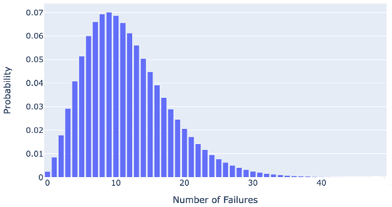
Figure 1.  The Probability mass function for negative binomial distribution⁽⁶⁾

It is important to mention that the negative binomial distribution is frequently employed to represent the number of failures before a specific number of successes in scenarios like waiting for the success in a series of Bernoulli trials. This distribution is applied in various fields, including probability theory, statistics, and actuarial science, to model scenarios where the timing of events is uncertain.

Negative Binomial Regression

Negative binomial regression is a type of regression analysis used when the dependent variable in a model is a count variable that follows a negative binomial distribution. This regression model is particularly suitable for situations where the data exhibit over dispersion, meaning the variance is greater than would be expected under a Poisson distribution. The negative binomial regression is an extension of the Poisson regression model, which is commonly used for count data. The Poisson distribution assumes that mean variance of the facts is same, which might not be the case in lots of real-international scenarios. Negative binomial regression relaxes this assumption through permitting the variance to be greater than the suggestion, providing a greater bendy version for count records.⁽⁷⁾

A logarithmic link function is used in negative binomial regression to simulate the relationship between the mean of the dependent variable and the independent variables. To represent the distribution of the dependent variable, one uses the probability mass function (PMF) of the negative binomial distribution. General negative binomial regression equation is:⁽⁸⁾

Ln(μ)the natural logarithm of mean of dependent variable, β₀, β₁,…β_k are the coefficients to be estimated,(x₁,…x_k)  are the independent variables.

Zero-Inflated Negative Binomial Model

A statistical model that incorporates components of the excess zero probability and the negative binomial distribution is called a Zero-Inflated Negative Binomial (ZINB) model. When there is an excess of zeros, or a disproportionate number of observations with zero counts, it is frequently used to examine count data.

In certain datasets, a substantial number of observations may have a count of zero due to a different process than the one generating the non-zero counts. The ZINB model accommodates this by having two components:

it deals with the excess zeros. It assumes that there are two processes contributing to the zero counts, a process that generates true zeros (structural zeros) and another process that may produce additional zeros (due to excessive zeros). This is typically modeled using a binary outcome variable indicating whether a count is zero or not.

This part models the non-zero counts and is similar to the negative binomial regression. It assumes that the non-zero counts follow a negative binomial distribution, similar to the Negative Binomial Regression model.

Let us propose that for each observation there are two possible states for the value that the hypothesized variable can take. Let us assume that in state (1), which is possible for the result to occur, the result is zero, and in state (2), which means that the first state will not occur.

Assuming that the chance of the first case happening is (π), and the chances of the second case occurring is complementary to the probability of the first possibility is(1-π)

Probability distribution function of the variable (x_i) will be:

So that (π_i) represents the logistic link function, (g(y_i)) is negative binomial distribution function and (μ_i) is average of the counting operations,

the zero-inflated regression variable (x_i, α) is the parameter by which the counting is done for the zero-inflated operations, which is:

The above equation assumes the logistic link function. The components of a negative binomial can include time (𝑡) and a set of variables bearing (𝑘) features, and then the variables (𝑋𝑘) are variables that are defined according to the following relationship:

It is the logistic function, with probability that the event will occur, Probability that the event will not occur is (1−𝜋) event is:

Estimation Methods

Statistical estimation methods play a pivotal role in extracting valuable information from data, enabling researchers to make inferences about underlying population parameters. Many statistical estimation methods can be used such the followings. In (MLE) parameters of the proposed model are estimated by the maximum likelihood function has divided the maximum likelihood into (4) parts, as follows:

The previous equation included (4) parts, which represents the logarithm of the Maximum likelihood. The division into (4) parts was used to facilitate taking the partial derivatives, so that each part could include one or more parameters, which facilitates taking. It is partial derivatives. as is known, the derivative of the sum of two functions is equal to the sum of their partial derivatives.

Where:

The partial derivatives of the previous maximum potential function with respect to β=μ_i will be:

r=1,2,..,k

Just as the derivation of the maximum likelihood function with respect to (γ=λ_i) will be:

r=1,2,..,m

The maximum likelihood estimators will be:

Log(L)=l(r,λ,ϑ,γ,ω)

Such that:

It can be noted that the five derivatives cannot be solved by direct methods (substitution) to find the estimators, so we resort to iterative numerical methods (Newton-Raphson method) to find these estimators.

According to this method, the estimates can be obtained by equating the expectations for the distribution with the sample moments and according to the sequence of relationships that connect them, and because there are five parameters that must be estimated, so the first five expectations are adopted as follows, (6). That is the first moment.

Moment Estimation Moment

The second moment

The third moment

The 4^th moment

The 5^th moment

The five moments of the sample are respectively:

Shrinkage Estimation Method

This method depends on reconciling more than one estimation method according to a formula based on the maximum benefit from their benefits and the maximum exclusion of the negatives that may be included in each individual estimator, according to the approved estimation method. This method is based on the following general formula.⁽¹⁰⁾

Where:

(p) represents the coefficient of contraction, which must initially be determined to be as small as possible.

(θ ̂₃) represents the estimator according to the downscaling method.

(θ ̂₁,θ ̂₂) represent the estimates of the two methods adopted in the reduction. The reduced estimator can be calculated according to the following steps.

The beginning

Assuming an initial value for the shrinkage parameter (p) and choosing the one closest to zero.

Calculating a new value for the shrinkage parameter according to the increment that is the lowest.

So that (ϵ) represents the amount of increase.

Calculate the value of the initial estimator of contraction according to the following:

Calculating the shrinkage estimator:

Calculate the absolute difference (ε) to be:

Where:

Then the initial estimated parameter is made equal to the new estimated parameter:

Return to step number (3):

Comparing criteria

In estimators the comparing criteria with the following formula:⁽¹⁰⁾

With: (δ represent Minimum absolute deference)

The mean square error will be:

The Simulation Experiments

It contains simulation experiments that were run with a predetermined sample size n and the goal of producing a negative binomial distribution, a specified zero inflation parameter (p), and a specified second parameter (β). The simulation experiments were represented according to the following data (inflation parameter (p=0,1, 0,5, 0,8) second parameter (β=1,2,3) sample size (n=20,50,100). It was also included applying each of the following estimation methods (11):

(MLE)  represent Maximum likelihood Estimation.

(MOM) represent Moment’s estimation method.

(SEM) represent Shrinkage estimation method.

RESULTS AND DISCUSSIONS

After carrying out the simulation experiments in accordance with the previous conditions and data, the following results was showed:

Table 1. The estimators’ values for () with various simulation parameters
β	p	n	MLEp	MOMp	SEMp	∅PMLE	∅PMOM	∅PSEM	δP	Best
1	0,1	20	0,168961	0,194794	0,142498	0,068961	0,094794	0,042498	0,042498	3
1	0,1	50	0,103053	0,10886	0,117193	0,003053	0,00886	0,017193	0,003053	1
1	0,1	100	0,109007	0,109623	0,100044	0,009007	0,009623	4,39E-05	4,39E-05	3
2	0,5	20	0,536971	0,579904	0,560116	0,036971	0,079904	0,060116	0,036971	1
2	0,5	50	0,516815	0,513078	0,500228	0,016815	0,013078	0,000228	0,000228	3
2	0,5	100	0,500454	0,502767	0,503179	0,000454	0,002767	0,003179	0,000454	1
3	0,8	20	0,807933	0,849636	0,868552	0,007933	0,049636	0,068552	0,007933	1
3	0,8	50	0,808105	0,811389	0,81719	0,008105	0,011389	0,01719	0,008105	1
3	0,8	100	0,80226	0,807264	0,804368	0,00226	0,007264	0,004368	0,00226	1

Figure 2. The absolute deference for (p) estimators with various simulation parameters

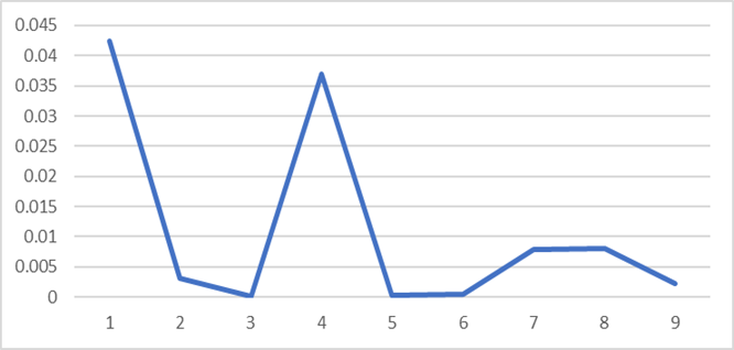
Figure 3. Minimum absolute deference for (p) estimators with various simulation parameters

Comparing the results showed that the lower value is due to the experiment with (p=0,1,n=100,β=1) with (δ_p=4,39E-05 ) and the value of the estimator is (p=0,100044) for the third estimation method (Shrinkage).

Table 2. The estimators’ values for (β) with various simulation parameters
β	p	n	MLEβ	MOMβ	SEMβ	∅βMLE	∅βMOM	∅βSEM	δβ	Best
1	0,1	20	0,149071	0,1406	0,190657	0,831039	0,805206	0,857502	0,805206	2
1	0,1	50	0,104329	0,119781	0,116456	0,896947	0,89114	0,882807	0,882807	3
1	0,1	100	0,108891	0,100745	0,10402	0,890993	0,890377	0,899956	0,890377	2
2	0,5	20	0,507527	0,514472	0,534417	1,463029	1,420096	1,439884	1,420096	2
2	0,5	50	0,506029	0,502748	0,509219	1,483185	1,486922	1,499772	1,483185	1
2	0,5	100	0,500361	0,503148	0,502957	1,499546	1,497233	1,496821	1,496821	3
3	0,8	20	0,802245	0,839313	0,834255	2,192067	2,150364	2,131448	2,131448	3
3	0,8	50	0,811645	0,816995	0,802542	2,191895	2,188611	2,18281	2,18281	3
3	0,8	100	0,806057	0,801502	0,80062	2,19774	2,192736	2,195632	2,192736	2

Figure 4. The absolute deference for (β) estimators with various simulation parameters

Figure 5. Minimum absolute deference for (β) estimators with various simulation parameters

Comparing the results showed that the lower value is due to the experiment with (p=0,1,n=20,β=1) with (δ_β=0,805206 ) and the value of the estimator is (β=0,1406) for the second estimation method (Moment).

Table 3. The MSE values for (p) with various simulation parameters
β	p	n	MLEP	MOMP	SEMP	MINMSEP	Best
1	0,1	20	0,162786	0,132258	0,122526	0,122526	3
1	0,1	50	0,074743	0,099796	0,046282	0,046282	3
1	0,1	100	0,069812	0,095392	0,042753	0,042753	3
2	0,5	20	0,050435	0,136336	0,061513	0,050435	1
2	0,5	50	0,036995	0,080467	0,069874	0,036995	1
2	0,5	100	0,037279	0,079979	0,061095	0,037279	1
3	0,8	20	0,010406	0,121469	0,117708	0,010406	1
3	0,8	50	0,015551	0,059009	0,076138	0,015551	1
3	0,8	100	0,008662	0,049734	0,06885	0,008662	1

Figure 6. Minimum mean square error for (p) estimators with various simulation parameters

Comparing the results showed that the lower value is due to the experiment with (p=0,8,n=100,β=3) with (MSE_p=0,008662 ) for the first estimation method (MLE).

Table 4. The estimators’ values for (β) with various simulation parameters
β	p	n	MLEβ	MOMβ	SEMβ	MINMSEβ	Best
1	0,1	20	0,928837	0,891416	0,915203	0,891416	2
1	0,1	50	0,84065	0,814525	0,865258	0,814525	2
1	0,1	100	0,831243	0,806141	0,857955	0,806141	2
2	0,5	20	1,498875	1,518362	1,49969	1,498875	1
2	0,5	50	1,469529	1,424487	1,441981	1,424487	2
2	0,5	100	1,463089	1,420404	1,440624	1,420404	2
3	0,8	20	2,213263	2,217481	2,182861	2,182861	3
3	0,8	50	2,201479	2,155738	2,1361	2,1361	3
3	0,8	100	2,19295	2,150794	2,132215	2,132215	3

Figure 7. Minimum mean square error for (β) estimators with various simulation parameters

Comparing the results showed that the lower value is due to the experiment with (p=0,1,n=100,β=1) with (MSE_p=0,806141) for the first estimation method (MOM).

As such, it is essential to acknowledge the limitations of research when studying and comparing various negative binomial regression models through simulations. Here are some potential constraints to consider:

CONCLUSIONS

The simulation experiments revealed that the sample size, initial parameter values, and the estimation method influenced the estimators, resulting in varying superiority rates for each estimation method. For instance, the percentage for MLE was 70 %, for MOM it was 30 %, and for SEM it was 0 % for the minimum absolute deference criteria and the () estimator. For MLE, the percentage was 12 %, for MOM it was 44 %, and for SEM it was 44 % for the minimum absolute deference criteria and the () estimator. For MLE, the percentage was (67 %), for MOM, the percentage was (42 %), and for SEM, the percentage was (33 %) for mean square error criteria and (11 %) estimator. For MLE, the percentage was (11 %), for MOM, the percentage was (56 %), and for SEM, the percentage was (33 %) for mean square error criteria and (32) estimator.

BIBLIOGRAPHIC REFERENCES

1. Neamah, M. W., & Raheem, S. H. (2021). Comparing Poisson Regression via Negative Binomial Regression for Modeling Zero-Inflated Data. International Journal of Agricultural & Statistical Sciences, 17(1).

2. AL-Mosawy, Z. A. A., & AL-Tai, A. H. H. (2023). Compare some Estimation Methods for Zero-Inflated Poisson Regression Models With Simulation. International Journal of Nonlinear Analysis and Applications, 14(1), 1787-1793.

3. da Silva, A. R., & de Sousa, M. D. R. (2023). Geographically Weighted Zero-Inflated Negative Binomial Regression: A general Case for Count Data. Spatial Statistics, 58, 100790.

4. Kadhim MT, Chilab AN. The effect of the formal organizer strategy on the achievement and visual thinking skills of first-year intermediate female students in social studies subject. Salud, Ciencia y Tecnología - Serie de Conferencias [Internet]. 2024 Jan. 1 [cited 2024 Aug. 21];3:962. Available from: https://conferencias.ageditor.ar/index.php/sctconf/article/view/829

5. He, Q., & Huang, H.-H. (2024). A Framework of Zero-Inflated Bayesian Negative Binomial Regression Models for Spatiotemporal Data. Journal of Statistical Planning and Inference, 229, 106098.

6. Hilbe, J. M. (2011). Negative Binomial Regression: Cambridge University Press.

7. Saengthong, P., Bodhisuwan, W., & Thongteeraparp, A. (2015). The Zero Inflated Negative Binomial–Crack Distribution: Some Properties and Parameter Estimation. Songklanakarin J. Sci. Technol, 37(6), 701-711.

8. Schmeiser, B. (1990). Simulation Experiments. Handbooks in Operations Research and Management Science, 2, 295-330.

9. Welch, P. D. (1983). The Statistical Analysis of Simulation Results. The Computer Performance Modeling Handbook, 22, 268-328.

10. Yu, D., Huber, W., & Vitek, O. (2013). Shrinkage Estimation of Dispersion in Negative Binomial Models for RNA-Seq Experiments with Small Sample Size. Bioinformatics, 29(10), 1275-1282. 

11. Zhou, M., Li, L., Dunson, D., & Carin, L. (2012). Lognormal and Gamma Mixed Negative Binomial Regression. Paper presented at the proceedings Of The... International Conference on Machine Learning. International Conference on Machine Learning.

FINANCING

No financing.

CONFLICT OF INTEREST

None.

AUTHORSHIP CONTRIBUTION

Conceptualization: Zahraa AbdulAmeer Ali AL-Mosawy, Nadiha Abed Habeeb.

Drafting - original draft: Zahraa AbdulAmeer Ali AL-Mosawy, Nadiha Abed Habeeb.

Writing - proofreading and editing: Zahraa AbdulAmeer Ali AL-Mosawy, Nadiha Abed Habeeb.