doi: 10.56294/sctconf2024.1399

ORIGINAL

Chemical bonding in the quantum and classical models

Enlace químico en los modelos cuántico y clásico

Lahbib ABBAS¹ *, Lahcen BIH² *, Abdessamad MEZDAR¹ *, Khalid SELLAM³ *, Ilyas. JALAFI⁴ *, Zahra RAMZI⁵ *

¹Moulay Ismail University Meknes, Faculty of Science and Technology, Chemistry department. Er-Rachidia, Morocco.

²Moulay Ismail University Meknes, National School of Arts and Crafts. Meknes, Morocco.

³Moulay Ismail University Meknes, Faculty of Science and Technology Er-Rachidia, Biology department. Morocco.

⁴Mohamed 1st University Oujda, Multidisciplinary Faculty of Nador, Chemistry department. Nador, Morocco.

⁵Cadi Ayyad University, Faculty of Sciences Semlalia, Chemistry department. Marrakech, Morocco.

Cite as: G Abbas L, Bih L, Abdessamad Mezdar AM, Sellam K, Jalafi I, Ramzi Z. Chemical bonding in the quantum and classical models. Salud, Ciencia y Tecnología - Serie de Conferencias. 2024; 3:.1399. https://doi.org/10.56294/sctconf2024.1399

Submitted: 16-05-2024                   Revised: 26-09-2024                   Accepted: 28-11-2024                 Published: 29-11-2024

Editor: Prof. Dr. William Castillo-González

Corresponding Author: Lahbib ABBAS *

ABSTRACT

Many questions arise when writing reaction mechanisms, and therefore require answers for which the molecular formulas of the different species, reagents or intermediates, conform to the rules of classical and quantum models for the construction of different species, and show single, double or triple bonds, non-bonding doublets, electron vacancies and charges, as well as mesomeric forms where appropriate.

The linear combination of atomic orbitals LCAO provides a visual representation of the energy levels associated with the different molecular orbitals formed from Atomic Orbitals (AO). LCAO is crucial for understanding the stability of molecules and the types of bonds they can form. Molecular Orbitals (MO) can be classified into two broad categories: bonding orbitals and antibonding orbitals.

The quantum model is particularly well suited to describing diatomic molecules. It can help explain, for example, why some molecules exist in nature and others does not, such as rare gas and alkaline-earth molecules, the relative strength of chemical bonds, and the origin of certain physical properties such as the dipole moment and magnetism of molecules.

The aim of this work is to compare the representation of chemical species between the quantum model (molecular orbital and hybridization theories) and the classical model (Gillespie theories and the systematic method of representing a molecule).

Keywords: Chemical Bonding; Atomic Orbital; Molecular Orbital; Linear Combination of Atomic Orbitals; Bonding Orbitals; Antibonding Orbitals.

RESUMEN

Al escribir los mecanismos de reacción surgen muchas preguntas, por lo que se requieren respuestas para las que las fórmulas moleculares de las diferentes especies, reactivos o intermedios, se ajusten a las reglas de los modelos clásicos y cuánticos para la construcción de diferentes especies, y muestren enlaces simples, dobles o triples, dobletes no enlazantes, vacantes y cargas electrónicas, así como formas mesoméricas cuando proceda.

La combinación lineal de orbitales atómicos LCAO proporciona una representación visual de los niveles de energía asociados a los diferentes orbitales moleculares formados a partir de orbitales atómicos (AO). LCAO es crucial para comprender la estabilidad de las moléculas y los tipos de enlaces que pueden formar. Los orbitales moleculares (MO) pueden clasificarse en dos grandes categorías: orbitales de enlace y orbitales antienlace. El modelo cuántico es especialmente adecuado para describir moléculas diatómicas. Puede ayudar a explicar, por ejemplo, por qué algunas moléculas existen en la naturaleza y otras no, como los gases raros y las moléculas alcalinotérreas, la fuerza relativa de los enlaces químicos y el origen de ciertas propiedades físicas como el momento dipolar y el magnetismo de las moléculas.

El objetivo de este trabajo es comparar la representación de las especies químicas entre el modelo cuántico (teorías de los orbitales moleculares y de la hibridación) y el modelo clásico (teorías de Gillespie y método sistemático de representación de una molécula).

Palabras clave: Enlace Químico; Orbital Atómico; Orbital Molecular; Combinación Lineal de Orbitales Atómicos; Orbitales Enlazantes; Orbitales Antienlazantes.

INTRODUCTION

Lewis structures are insufficient to interpret the existence of the H₂⁺ ion, in which a bond is formed by a single electron, and to explain the paramagnetic of oxygen. In no case do they provide any information about the energy levels of electrons in molecules or ions. A more detailed description of bonds, which accounts for the electronic properties of molecules, is based on the theory of molecular orbitals.^(1,2)

We know that for an atom, an electron of given energy in the field exerted by the nucleus is described by a wave function called an atomic orbital. The theory of molecular orbitals considers that in a molecule an electron is subject to the field exerted by the electrons and all the nuclei linked together and that it is described by a wave function called a molecular orbital. Each molecular orbital corresponds to an energy level and can describe a maximum of two electrons with opposite spins. The expressions for the different molecular orbitals can only be determined rigorously in the case of a single-electron diatomic system (e.g. H₂⁺). In other cases, we use an approximation that identifies a molecular orbital with a linear combination of valence atomic orbitals of atoms linked together, a method known as LCAO: "Linear Combination of Atomic Orbitals". The valence atomic orbitals that contribute to the formation of molecular orbitals are those that have similar energies and the same symmetry elements; they are those that have a good overlap of their probability of presence domains.^(3,4,5) The Schrödinger equation is solved by taking into account the following 3 considerations:

The Born-Oppenheimer approximation, which assumes that nuclei are immobile;

In the case of a polyatomic molecule, made up of a chain of atoms A, B, C, ......,J , the poly-electronic wave function or a molecular orbital (M.O.) Ψmol is thus obtained by a linear combination of the interacting atomic orbitals φA, φB, φC, ...., φJ written:

Ψmol = c_Aφ_A + c_B  φ_B + c_C  φ_C + ……+c_J  φ_J

Where:

· c_i: being the weighting coefficient.

· φ_i: atomic orbital function.

The simplest solution of a molecular orbital was proposed by Mulliken: it is a linear combination of valence atomic orbitals φi known by the abbreviation LCAO:

Ψmol = ∑_iC_iφ_i

The coefficients here are determined according to the conditions:

· The energy of the system is minimal.

· The Ψmol M.O are normalized.

· M.O. Ψmol are orthogonal.

The CLAO method is an approximation in which a molecular orbital is a linear combination of atomic orbitals:

Ψmol = ∑_iC_iφ_i

This may seem laborious with atoms that have many atomic orbitals, but we will make an additional approximation by taking into account only the valence AO.

If we consider the H₂⁺ molecule (the simplest) we obtain:

ΨH₂⁺ = C₁φ₁+ C₂φ₂

In this case we will say that the 2 OAs φ₁ et φ₂ interact to lead to molecular orbitals

These MO are solutions of Schrödinger's equation: Ĥ𝜓 = ε𝜓

With Ĥ : single electronic Hamiltonian operator and ε ∶ and the energy of the molecular orbital

The Hamiltonian operator being linear we can multiply left and right by 𝜓 and develop all this:

Ĥ(C₁φ₁+ C₂φ₂)² = ε(C₁φ₁+ C₂φ₂)²

C₁² φ₁Ĥφ₁ + C₁² φ₂ Ĥφ₂+ 2c₁ c₂ φ₁Ĥφ₂= ε(C₁² φ₁ φ₁ + C₁² φ₂ φ₂+ 2c₁ c₂ φ₁ φ₂)

We integrate all this on the volume and adopt a simplified writing style.

𝛼𝑖 = ∭ φ_iĤφ_i 𝑑𝜏 volume: Coulomb integral

𝛽𝑖𝑗 = ∭ φ_iĤφ_j 𝑑𝜏 volume: resonance integral (with I ≠ j)

𝑆𝑖𝑗 = ∭ φ_i φ_j 𝑑𝜏 volume: recovery integral (with i ≠ j)

If S_ii = S_jj = 1 because of the normalization condition which tells us that an OA is indeed found on the volume around the atom.

Since the two atoms (1 and 2) are identical, we can simplify the writing:

The result is: C₁² α₁ + C₂² α₂ + 2c₁ c₂ β₁₂ = ε (C₁² + C₂² + 2c₁ c₂ S₁₂)

The energy and coefficient values are determined by assuming that the coefficient values are those that minimize the energy of the OM: soit ∂ε/∂c1 = ∂ε/∂c2 = 0

This gives us a system of 2 equations with 3 unknowns:

(α - ε) c1 + (β – ε S) c2 = 0

β - εS) c1 + (α - ε) c2 = 0

For a non-trivial solution where c1 = c2 = 0, the secular determinant of the matrix below must be zero:

(α - ε &β - εS)/ (β - εS &α - ε)|= 0

We then obtain (α - ε)² - (β - εS)² = 0 which gives us a 2nd degree equation in 𝜀 whose solutions are:

ε₁ = (α + β)/(1 + S ) et ε₂ = (α - β )/(1-S)

Here we can see that the interaction of two atomic orbitals results in the construction of 2 molecular orbitals. This result can be generalized: the interaction of n atomic orbitals results in the construction of n molecular orbitals.

The LCAO method can be used to obtain the binding and non-binding molecular wave functions and determine the corresponding energy levels.⁽⁶⁾ If the wave functions associated with the two atomic orbitals have the same sign in the inter-nuclear region, where they overlap, the overlap between orbitals is said to be constructive. Such overlap increases the probability of finding an electron in this region of space. Molecular orbitals formed from a constructive overlap, if occupied by electrons, help to link two atoms. They are therefore called bonding orbitals. A binding OM is characterized by an energy lower than the energies of the AO of which it is made up (figure 1).^{(7,8,9,10,11)} On the other hand, if the wave functions associated with the two atomic orbitals are of opposite sign in the internuclear region, the overlap between orbitals is said to be destructive. Such overlap reduces the probability of finding an electron in this region of space. OMs formed from destructive overlap are called anti-bonding orbitals and, if occupied by electrons, contribute to destabilization of the chemical bond. An anti-bonding OM is characterized by a higher energy than the energies of the AO of which it is made up, and has a nodal plane perpendicular to the internuclear axis. Anti-bonding orbitals are marked by asterisks (*) or (u) in the OM diagram (figure 1).^(12,13,14)

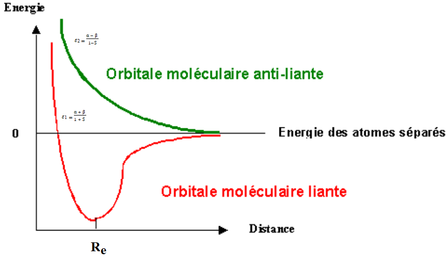
Figure 1. Energies of bonding and non-bonding molecular orbitals as a function of internuclear distance^(12,13,14)

If the overlap between two atomic orbitals is zero, either because they don't overlap, or because a constructive overlap in one region exactly compensates for a destructive overlap in another region, then the OM is called a non-bonding orbital. A non-bonding OM has the same energy as the AO that make it up.

It is convenient to represent, on the same diagram, the energy levels of the valence atomic orbitals of separate atoms and of the resulting bonding and non-bonding molecular orbitals, for a distance between the nuclei equal to the length of the bond.

The rules for constructing molecular orbital diagrams:^{(15,16,17,18,19,20)} (1) interacting A.O have comparable energies (typically ΔE < 13 eV); (2) A.O only interact if their overlap is non-zero; (3) the number of M.O formed is always equal to the number of interacting A.O. .A. that interact; (4) The destabilization of an anti-binding M.O. is greater than the stabilization of the associated binding M.O.; (5) The relative position of the M.O. depends on the energies of the starting A.O.s; (6) A.O. only interact if they have the same symmetry.

Some values for the AO energies of a few chemical elements are shown in table 1 after.^{(21,22,23,24,25,26)}

Table 1. Calculated energies of some OA (in eV)
	Element	H	He
Orbital energy in the neutral atom (eV)	Z	1	2
	1s	-13,598	-24,588
	Element	Li	Be	B	C	N	O	F	Ne
	Z	3	4	5	6	7	8	9	10
	1s	-57,875	-114,34	-192,25	-288,23	-403,78	-538,25	-692,45	-869,53
	2s	-5,3917	-9,3226	-12,930	-16,590	-20,330	-28,720	-37,213	-47,735
	2p			-8,2980	-11,260	-14,534	-13,618	-17,423	-21,565
	Element	Na	Mg	Al	Si	P	S	Cl	Ar
	Z	11	12	13	14	15	16	17	18
	1s	-1074,4	-1307,3	-1564,1	-1844,1	-2148,3	-2475,8	-2829,1	-3206,2
	2s	-66,020	-92,180	-121,46	-154,04	-191,40	-232,10	-276,60	-324,20
	2p	-33,520	-53,773	-76,753	-103,71	-135,12	-168,10	-206,35	-247,74
	3s	-5,1391	-7,6462	-10,620	-13,460	-16,150	-20,200	-24,540	-29,240
	3p			-5,9858	-8,1517	-10,487	-10,360	-12,968	-15,760

The dynamic orbital forces of diatomic molecules have been calculated for a number of diatomic molecules after.^{(27,28,30,31)}

Table 2. Dynamic orbital forces of homonuclear diatoms in atomic units (Hartree/Bohr); a positive value indicates a binding OM and vice versa (after)
OM	H2	Li2	N2	O2	F2	P2	S2	Cl2
1σ1s	0,164	0,010	0,394	0,492	0,343	0,115	0,180	0,156
1σ2s			- 0,176	- 0,201	- 0,167	- 0,076	- 0,074	- 0,063
σz			0,047	0,111	0,215	- 0,008	0,039	0,096
πx			0,238	0,209	0,136	0,072	0,095	0,068
πy				- 0,199	- 0,125		- 0,053	- 0,056

AB molecules are asymmetrical, the A.O. of atoms A and B are different and x(B) ¹ x(A). The atomic orbitals of one of the atoms may exhibit s-p interactions. It will be assumed that the results obtained for homo-nuclear A₂ molecules can be at least qualitatively generalized to hetero-nuclear AB molecules. We'll also assume the following results:^{(32,33,34,35)}

The most electronegative B atom, for example (x(B) > x(A)), weighs more heavily in a bonding OM, and vice versa for the least electronegative A atom in an anti-bonding OM.

As a general rule, the most electronegative atoms that strongly retain their electrons have lower-energy (more stable) atomic orbitals for a given level than less electronegative atoms.

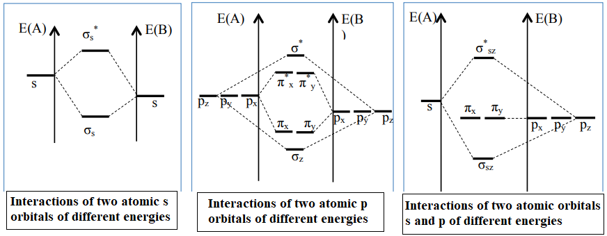
Figure 2. Molecular orbital energies of AB hetero-nuclear molecules⁽²⁾

Species with single electrons are called paramagnetic, and those without are called diamagnetic.

The overall bonding strength or bonding index is defined:

This is the number of single electrons divided by two (the single electrons involved in bond formation, divided by two because the bond is made up of two electrons).

or, by the following relationship:

Il=(n_é+n_é*)/2

Where:

· n_e (bonding).

· n_e* (non-bonding) represent the number of electrons in bonding and non-bonding molecular orbitals, respectively.

Non-bonding electrons are not taken into account when calculating bond order, as these electrons are not involved in the molecule's bond formation.

The bond index provides information on the strength of the bond. The higher it is, the stronger the bond and the shorter its length. If it is zero, no bond can be formed and the molecule cannot exist.

Classic model: Systematic Lewis representation method

The systematic method for constructing Lewis representations of species is based on the seven steps cited by Abbas et al.⁽³⁶⁾. The semi-developed representation of the O₂ molecule according to the systematic method of Lewis representations⁽³⁶⁾ is given as follows:

Case of the molecule O₂

Step 1

n_EV (O₂) = 2n_EV (O) - 0

Z(O) = 8 hence [He] 2s² 2p⁴; n_EV (O)=6

n_EV (O₂)= 2× 6 = 12

Step 2

n_D (O₂) = ½ ×n_EV(O₂) = 12⁄2 = 6 binding and non-binding doublets.

Step 3

n_D.N.L (O₂) = 2 n_D.N.L (O₂) - 0

n_D.N.L (O₂) = 2 × 2 – 0 = 4 non- bonding doublets.

Step 4

n_DL (O₂)= n_D(O₂) – n_DNL(O₂) so n_DL (O₂) = 6 - 4 = 2 bonding doublets.

Step 5

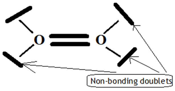
Figure 3. Molecule O₂E₄

The V.S.E.P.R formulation is expressed as follows: AXnEn^':

O: central atom.

1 O atom covalently bonded to the O atom and n=2 their number.

E: non-bonding doublets and 4 their number on each oxygen atom.

The Gillespie type of molecule is therefore O₂E₄ and the basic geometry triangular.

Step 6

C.F (O) = n_E.V(O in isolated state) - n_E.V (O linked to the building) = 6-6 = 0

Step 7

Build the structure using the systematic method: Same structure as described above.

Case of the molecule N₂

In the following we present the construction of Lewis representations according to the systematic method of the N₂ molecule.⁽³⁶⁾

Step 1

n_EV(N₂) = 2n_E.V(N) - 0

Z(N) = 7 hence [He] 2s2 2p3; n_E.V (N) =5

n_EV(N₂)= 2×5 = 10

Step 2

n_D(N₂) = ½ ×n_EV(N₂) = 10⁄2 = 5 binding and non-binding doublets

Step 3

n_DNL(N₂) = 2 n_D.N.L(N) - 0

n_D.N.L (N2) = 2 × 1 – 0 = 2 non-bonding doublets

Step 4

n_DL(N₂)= n_D(N₂) –  N_DNL(N2) so n_DL(N₂) = 3 -2 = 3 Binding doublets

Step 5

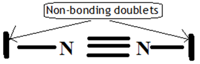
Figure 4. Molecule N₂E₂

The V.S.E.P.R formulation is expressed as follows: AXnEn^':

N: central atom

1 N atom covalently bonded to N atom and n=2 their number.

E: non-bonding doublets and 2 their number on the valence layer of each N atom.

So the Gillespie type of molecule is N₂E₂ and the geometry is linear.

Step 6

C.F (N) = n_E.V (N in isolated state) - n_E.V(N linked to the building) = 5-5 = 0

Step 7

Build the structure using the systematic method: Same structure as described above.

Case of the CO molecule

In this section, we present the construction of Lewis representations using the systematic method for the CO.⁽³⁶⁾

Step 1

n_EV(CO) = n_EV(C) +  n_EV(O)-0

Z(O) = 8 hence [He] 2s2 2p4; n_EV(O) =6 et Z(C) = 1 hence 2s² 2p²; n_EV(C)=4

n_EV(CO)= 4 + 6 = 10

Step 2

n_D(CO) = ½ × n_EV(CO) =  10⁄2 = 5 binding and non-binding doublets

Step 3

n_DNL(CO) = n_D.N.L(O) + n_D.N.L(C)-0

n_DNL(CO) = 2 + 1 – 0 = 3 non-bonding doublets

Step 4

n_DL(CO)= n_D(CO) –  n_D.N.L(CO) so n_D.L(CO) = 5 -3 = 2 Doublets liants

Step 5

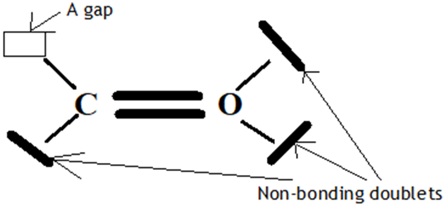
Figure 5. Molecule COE₃

The V.S.E.P.R formulation is expressed as follows: AXnEn′

O: central atom

1 C atom covalently bonded to the O atom and n=1 their number.

E: non-bonding doublets and 3 their number, 2 on the valence layer of the O atom and one on the carbon atom.

The Gillespie type of molecule is therefore COE₃ and the basic geometry triangular.

Step 6

C.F (O) = n_E.V (O in isolated state) - n_E.V (N linked to the building) = 6-6 = 0

C.F (C) = n_E.V (C in isolated state) - n_E.V (C linked to the building) = 4-4 = 0

Step 7

Build the structure using the systematic method: Same structure as described above.

Case of the HF molecule

In this section we present the construction of Lewis representations according to the systematic method of the HF molecule.⁽³⁶⁾

Step 1

n_EV(HF) = n_EV(H) + n_EV (F)-0

Z(F) = 9 hence [He] 2s² 2p⁵; n_EV(F) =7 and Z(H) = 1 hence 1s1; nEV(H) =1

n_EV(HF) = 1×1 + 7  = 8

Step 2

n_D (HF) = ½ ×n_EV(HF)= 8⁄2 = 4 binding and non-binding doublets.

Step 3

n_DNL (HF) = n_D.N.L (F) + n_D.N.L(H)-0

n_DNL (HF) = 3 + 0 – 0 = 3 non-bonding doublets.

Step 4

n_DL(HF)= n_D(HF) – n_DNL(HF) so n_DL(HF) = 4 -3 = 1 bonding Doublets.

Step 5

Figure 6. Molecule HFE₃

The V.S.E.P.R formulation is expressed as follows: AXnEn′

F: central atom.

1 H atom bonded to F atom by covalent bond and n=1 their number.

E: non-bonding doublets and 3 their number on the valence layer of atom F.

The Gillespie type of molecule is therefore HFE₃ and the basic geometry tetrahedral.

Step 6

C.F (F) = n_EV (F in isolated state) - n_EV(F linked to the building) = 7-7 = 0

C.F (H) = n_EV (H in isolated state) - n_EV(H linked to the building) = 1-1 = 0

Step 7

Building the structure using the systematic method: Same structure as described above.

Case of the H₂O molecule

In the following, we present the construction of Lewis representations using the systematic method for the H₂O molecule.⁽³⁶⁾

Step 1

n_EV (H₂O) = 2n_EV(H) + n_EV (O)-0

Z(O) = 8 hence [He] 2s² 2p⁴; n_EV(O) =6; Z(H) = 1 hence 1s¹; n_EV(H) =1

n_EV (H₂O)= 2×1 + 6 = 8

Step 2

n_D(H₂O) = ½ ×n_EV H₂O = 8⁄2 = 4 binding and non-binding doublets.

Step 3

n_DNL (H₂O) = n_D.N.L(O) + 2 n_D.N.L(H)-0.

n_DNL(H₂O) = 2 + 2 × 0 – 0 = 2 non-bonding doublets.

Step 4

n_DL(H₂O)= n_D(H₂O) – n_DNL)(H₂O) so n_DL(H₂O) = 4 -2 = 2 bonding doublets.

Step 5

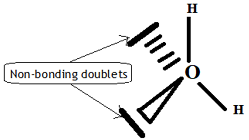
Figure 7. Molecule H₂OE₂

The V.S.E.P.R formulation is expressed as follows: AXnEn′

O: central atom.

2 H atoms linked to the O atom by covalent bond and n=2 their number.

E: non-bonding doublets and 2 their number on the valence layer of the O atom.

The Gillespie type of molecule is therefore H₂OE₂ and the basic geometry tetrahedral.

Step 6

C.F (O) = n_EV(O in isolated state) - n_EV(N linked to the building) = 6-6 = 0

C.F (H) = n_EV(H in isolated state) - n_EV(H linked to the building) = 1-1 = 0; no charge for both hydrogens.

Step 7

Building the structure using the systematic method: Same structure as described above.

Among the limitations and shortcomings of the classical model, (1) it doesn't explain the paramagnetic character of some molecules, (2) it doesn't give an idea of the nature and strength of the bond (dipole moment, energy and bond length). This model is complemented by the quantum model.

Quantum model: Linear combination of atomic orbitals

Case of the molecule O₂

The OM diagram shown in figure 3 can be used to interpret the paramagnetism of O₂, as well as some experimental properties (dissociation energy, bond length, etc.). The valence electrons of oxygen are: (2s)² (2p)⁴. In the O₂ molecule, each oxygen atom contributes 8 electrons. Oxygen's 16 electrons are placed in molecular orbitals according to the following three rules:

· Klechkowski's rule: lower-energy orbitals are filled first, then higher-energy orbitals.

· Pauli's exclusion principle: a molecular orbital can only contain a maximum of two electrons with opposite spins.

· Hund's rule: when filling several OM of the same energy, we first place one electron in each orbital, with the same spin for each, before placing two electrons with opposite spins in the same orbital.

The energy difference between the valence orbitals (2s) and (2p) of two oxygen atoms is of the order of 15,102 eV.^{(21,22,23,24,25,26)} (table 1), so the interaction between (2s) and (2p) is negligible. When two oxygen atoms interact, we will consider only the interactions: 2s-2s and 2p-2p. The interaction between the two 2s OAs gives two σ-symmetric OM, a binding OM denoted σ_2s and an anti-binding OM denoted σ_2s*. The interaction between the two 2p_z OA gives two σ-symmetry OM, a binding OM noted σ_z and an anti-binding OM noted σ_z*. The 2px OAs will interact to form the π_x and π_x* OM, and the 2p_y OA will interact to form the π_y and π_y* OM. However, one point is unsatisfactory in this diagram (figure 8): for 2s OA in O₂, we find that the anti-binding σ_2s* is only very weakly destabilized compared to the OA levels (0,9 eV) and that the binding OM is strongly stabilized (10,8 eV). For 2p OA in O₂,: we find in OM σ_z a coefficient of 2p equal to 3,9; that of σ_z* being equal to -20,1; that of π_x, π_y being equal to 2,9 and that of π_x* π_y*  being equal to -3,3. The axial overlap between OA of σ symmetry is greater than the lateral overlap between OA of π symmetry. The energy gap between σ and σ* orbitals will therefore be stronger than that between π and π* orbitals (based on the energies quoted in table 2.^{(27,28,29,30,31)}. Figure 8 shows the energy diagram for the O₂ molecule.

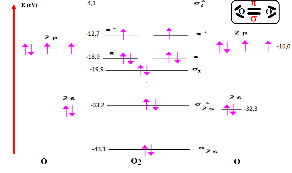
Figure 8. Energy diagram of the molecule O₂

According to figure 3, the electronic configuration of the OMs of O2 is as follows:

(σ_1s)² (σ_1s*)² (σ_2s)² (σ_2s*)²(σ_z)² (π_x π_y)⁴ (π_x* π_y*)²

The diagram (figure 3) for oxygen shows 2 unpaired electrons, indicating that the molecule is paramagnetic. The great success of this theory of molecular orbitals lies partly in the fact that it explains what has been observed experimentally and could not be explained by the classical model.

The energy order of the OM in O₂ is the same for F₂ and Ne₂, and also for the 3rd period molecules S₂, Cl₂ and Ar₂^{(21,22,23,24,25,26)} (tables 1 and 2).

The oxygen bonding index is 2 (the number of non-bonding electrons is eight, bonding and non-bonding electrons is four).

The dioxygen triplet bond:

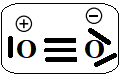
Figure 9. Dioxygen triplet bond

Can thus be described as one"classical" σ bond and two π half-bonds, each half-bond resulting from a two-center, three-electron interaction (2c-3e) as suggested by Linus Pauling.⁽³⁷⁾ The formal bond order is always equal to 2.

The most convenient representation for O₂ is the most stable one that respects the Octet rule, so the double bond.

Figure 10. Dioxygen double bond

Is the most representative of O₂. Single:

Figure 11. Dioxygen single bond

And triple:

Figure 12. Dioxygen triple bond

Bonds are not stable, because they don't respect the Octet rule, and because the electronic configuration of the OMs in O₂ creates single electrons in the π_x* and π_y* orbitals. These electrons destabilize the structure, so the O₂ molecule must not have a triple bond between separate O₂ atoms. It must have either I_l =1 or 2. But I_l = 1 is not stable, hence the most representative chemical bond of O₂ is the one with a bond order equal to two.

For the O₂ molecule, E_diss dissociation energies and R_e experimental bond lengths are available to clarify certain orbital characteristics. These two parameters are linked: the presence of a bonding electron increases the dissociation energy and shortens the bond, and vice versa. The oxygen molecule has a dissociation energy and bond length as shown in table 3.

The OM electronic configuration, bond lengths and energies, bond order and magnetism of some molecules and ions are shown in table 3 below:

Table 3. Some bond lengths (pm), bond energies (kJ/mol), OM electronic configuration, bond order and magnetism^(38,39)
Species	Electronic configuration MO	Il	Re (pm)	Ediss (Kj/mol)	Magnetism
O≡O		3
O=O	(σ1s)^2 (σ*1s)^2 (σ2s)^2 (σ*2s)^2 (σz)^2 (πxπy)^4 (π*xπ*y)^2= [O2]	2	121	490	para
O-O		1	147	143
O2^+	(σ1s)^2 (σ*1s)^2 (σ2s)^2 (σ*2s)^2 (σz)^2 (πxπy)^4 (π*x)^1	2,5	112	652	para
O2^2+	(σ1s)^2 (σ*1s)^2 (σ2s)^2 (σ*2s)^2 (πxπy)^4(σz)^2 = [N2]	3	107	625	dia
O2^-	(σ1s)^2 (σ*1s)^2 (σ2s)^2 (σ*2s)^2 (σz)^2 (πxπy)^4 (π*xπ*y)^3= [O2](πx*)	1,5	128	396	para
O2^2-	(σ1s)^2 (σ*1s)^2 (σ2s)^2 (σ*2s)^2 (σz)^2 (πxπy)^4 (π*xπ*y)^4= [F2]	1	149	493	dia^**
Note:^**From the electronic configuration of the O2^2- ion is (σ1s)^2 (σ*1s)^2 (σ2s)^2 (σ*2s)^2 (σz)^2 (πxπy)^4 (π*xπ*y)^4= [F2], we can deduce that the magnetism of O2^2- is diamagnetic.

It's fairly easy to predict the evolution of the O-O distance when electrons are added or removed. If one or two electrons are stripped from the π_x* or π_y* OMs of O₂, anti-bonding OM are depopulated, strengthening the bond (table 3). The distance shortens from O₂ to O₂⁺ or from O₂ to O₂²⁺, also, binding energy and binding index increase and magnetism disappears from O₂ to O₂⁺ or from O₂ to O₂²⁺ (table 3), conversely when we add one or two electrons in these same OMs, we fill anti-binding OMs, which weakens the bond. The distance lengthens from O₂ to O₂^- or from O₂ to O₂^2- (table 3), the binding energy and binding index decrease and magnetism disappears from O₂ to O₂^- or from O₂ to O₂^2-. In addition, some O₂⁺ excited states corresponding to ionization from deeper OMs have been experimentally characterized. The corresponding variations in bond lengths, in sign and relative value, help to clarify the nature and importance of the binding/anti-binding character of these OMs (table 3). This confirms that σ_s; σ_z; π_x and π_y is binding, but that σ_z* is only weakly binding.

The systematic method for constructing Lewis representations⁽³⁶⁾ reveals an O=O double bond and four free pairs. It does not account for the total spin of the molecule, since all electrons are paired, so the total spin should be zero, whereas oxygen is paramagnetic. We can conclude that the classical model of the systematic method for constructing Lewis representations confirms and affirms the results we found with the quantum model of molecular orbital theory.

Case of the molecule N₂

The OM diagram given in figure 4 is used to interpret N₂ magnetism, as well as some experimental properties (dissociation energy, bond length, ...). In the case of the nitrogen molecule, each nitrogen atom contributes 7 electrons. Nitrogen's 14 electrons are placed in molecular orbitals according to the filling rules described above.

The energy difference between the (2s) and (2p) valence orbitals of two nitrogen atoms is of the order of 5,8 eV (table 1).^{(21,22,23,24,25,26)}The 2s-2p gap is now only 13 eV, and the 2s-2p interaction becomes more important. When two nitrogen atoms interact, the valence electrons are: (2s)²(2p)³, so we'll consider the interactions: 2s-2s; 2s-2p and 2p-2p. Interactions between the four 2s and 2p_z OA therefore give four OM: σ_2s, σ_2s*, σ_z and σ_z*, two binding OM noted σ_2s and σ_z; two antibinding OM noted σ_2s* and σ_z*. The four OA of type 2p_x and 2p_y will interact to form the four OM: π_x, π_x*, π_y and π_y*. The most notable change that appears in the diagrams figure 4 corresponds to the destabilization of the σ_z OM formed by the interaction of the 2p_z OA, which leads to an inversion of the energy levels of the σ_z and π_x, π_y OM. According to this correlated diagram, it's mainly the 𝝅 bonds that are bonded, as they have a lower energy than the σ_z bond. Note that the σ_z* and σ_z OM have lost some of their anti-bonding and bonding properties, respectively, to approach non-bonding OM. For 2s OA in N₂, we find that the anti-binding σ_2s* is only weakly destabilized compared to the levels of the OA and that the binding OM is very strongly stabilized (15,9 eV). For the 2p OA in N₂: we find in OM σ_z a coefficient of 2p equal to 1,1; that of σ_z* being equal to -21,5. that of π_x, π_y being equal to 0,9 and that of π_x*, π_y* being equal to -16,5 (according to the energies quoted in table 2.^{(27,28,29,30,31)} The energy levels of M.O. σ_z and (π_x, π_y) are inverted. We also say that we have a correlated energy diagram. Figure 13 shows the energy diagram for the N₂ molecule.

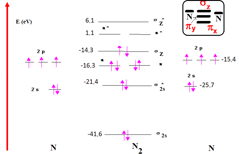
Figure 13. Energy diagram of the N₂ molecule

From figure 13, we deduce that the electronic configuration of the OMs of N₂ is as follows:

(σ_1s)² (σ*_1s)² (σ_2s)² (σ*_2s)² (π_xπ_y)⁴ (σ_z)²

We assume that the energy order of the OM in N is the same for the 2nd period molecules C₂ and B₂, and also for the 3rd period molecules Al₂, Si₂, P₂^{(21,22,23,24,25,26)} (table 1 and 2).

The N₂ molecule has no single electrons, it is diamagnetic, the bonding index of nitrogen is 3 (The number of non-bonding electrons is four, bonding electrons or anti-bonding electrons is six).^(15,16) We thus find the triple bond of the classical model: N ≡ N.⁽³⁶⁾

In the construction of the N₂ molecule of the classical model, the balance is a triple bond, i.e. three bonds: 1σ and 2π and two free pairs on the nitrogen atom, it becomes clear that the most representative bond of N₂ is the most stable one and one that respects the Octet rule, low bond energy and short bond length, and from the data in table 4, the triple bond that possess these standards. Whereas those equal to I_l = 1 or 2 do not present these conditions because, they do not respect the Octet rule and have a higher bond energy and a longer bond length compared to that of triple bond. This stability is found in the isoelectronic molecules of N₂: O₂²⁺ and: cyanide ion: CN^-.

Table 4. Some bond lengths (pm), bond energies (kJ/mol), OM electronic configuration, bond order and magnetism^(38,39)
Specie	Electronic configuration OM	Il	Re (pm)	Ediss (Kj/mol)	Magnetism
N≡N	(σ1s)^2 (σ*1s)^2 (σ2s)^2 (σ*2s)^2 (πxπy)^4(σz)^2 = [N2]	3	110	945	dia
N=N		2	125	418
N-N		1	145	170
N2^+	(σ1s)^2 (σ*1s)^2 (σ2s)^2 (σ*2s)^2 (πxπy)^4(σz)^1= [C2]( σz)^1	2,5	112	853	para
N2^2+	(σ1s)^2 (σ*1s)^2 (σ2s)^2 (σ*2s)^2 (πxπy)^4 = [C2]	2			dia
N2^-	(σ1s)^2 (σ*1s)^2 (σ2s)^2 (σ*2s)^2 (σz)^2 (πxπy)^4 (π*x)^1	2,5			para
N2^2-	(σ1s)^2 (σ*1s)^2 (σ2s)^2 (σ*2s)^2 (σz)^2 (πxπy)^4 (π*xπ*y)^2= [O2]	2			para
N2^3-	(σ1s)^2 (σ*1s)^2 (σ2s)^2 (σ*2s)^2 (σz)^2 (πxπy)^4 (π*xπ*y)^3	1,5			para
N2^4-	(σ1s)^2 (σ*1s)^2 (σ2s)^2 (σ*2s)^2 (σz)^2 (πxπy)^4 (π*xπ*y)^4= [F2]	1			dia

The OM electronic configuration, bond lengths and energies, bond order and magnetism of some species are shown in table 4 below:

It's fairly easy to predict the evolution of the N-N distance when electrons are added or removed. If one or two electrons are stripped from the σ_z OM of N₂, σ_z OM are depopulated, weakening the bond, decreasing the bond index (table 4). Binding strength decreases from N₂ to N₂⁺ or from N₂ to N₂²⁺, also, binding energy and binding index decrease and magnetism reappears from N₂ to N₂⁺ or disappears from N₂⁺ to N₂²⁺ (table 4), on the other hand, adding one or two electrons to these same OM fills anti-bonding OM, weakening the bond. Bond strength decreases from N₂ to N₂^- or from N₂ to N₂^2- (table 4), also, bond index decreases and magnetism appears from N₂ to N₂^- or from N₂ to N₂^2-.

The systematic method for constructing Lewis representations⁽³⁶⁾ reveals an N≡N triple bond and two free pairs. We can conclude that the classical model of the systematic method for the construction of Lewis representations confirms and affirms the results we found by the quantum model of molecular orbital theory.

Case of the CO molecule

In the case of the CO molecule, the atomic orbitals (AO) 2s(C) and 2p(C) are combined with the AO 2s(O) and 2p(O). This gives a total of eight AO, creating eight molecular orbitals (MO). OA 2s (O) has an energy of -32,3 eV, while OA 2p (C) is -11,4 eV. Given this large energy gap, these two OAs do not combine. The two OAs 2s(C) and 2s(O) will interact to form the two OM σ_2s and σ_2s*. (ΔE OA(2s(C)-2s(O)) < 13). The 2p_x oxygen atom level is non-binding and their energy is unaffected by molecule formation (table 1).^{(21,22,23,24,25,26)} Interactions between the two OA of 2p_z (C) and 2p_z (O) give two OM σ_z and σ_z*. and the two OA 2p_y (C) and 2p_y (O) will interact to form OM π_y and π_y*. For the 2s(C) OA, we find that the anti-binding σ_2s* is only very weakly destabilized compared to the (C) OA levels (0,7 eV) and that the binding σ_2s OM is strongly stabilized (10,1 eV). The most notable change shown in the diagram in figure 14 corresponds to the destabilization of the σz OM formed by the interaction of the 2p_z (C)- 2p_z (O) OA, resulting in an inversion of the σ_z and π_x, π_y OM energy levels. According to this correlated diagram it's mainly the 𝝅 bonds that are bound because they have a lower energy than the binding σ_z. Figure 14 shows the energy diagram for the CO molecule.

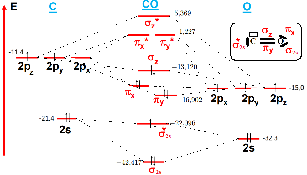
Figure 14. Energy diagram of the CO molecule

The electronic configuration of the CO molecule is:

(σ_1s)² (σ_1s*)² (σ_2s)² (σ_2s*)² (π_x)² (π_y)² (σ_z)²

The CO molecule has no single electrons, is diamagnetic and has a bond index of 2 (the number of non-bonding electrons is six, bonding electrons and non-bonding electrons is four).^(15,16) We thus find the double bond of the classical model: C = O.⁽³⁶⁾

The CO triplet bond:

Figure 15. CO triplet bond

Can thus be described as one σ bond and two π bonds. This bond has the lowest bond energy and shortest bond length (see table 5), and as suggested by Werner Kutzelnigg et al.⁽⁴⁰⁾.

The semi-developed formulas for CO are single bond: (I_l=1)

Figure 16. CO single bond

Double bond: (I_l=2)

Figure 17. CO double bond

Triple bond: (I_l=3)

Figure 18. CO triple bond

The most representative form is the most stable one, respecting the octet rule. Consequently, from these semi-developed formulas, single and triple bonds of CO are not stable, so the double bond as described above in the construction of the CO molecule of the classical model is the most stable.

In the case of CO ((C) = 2,55 and (O) = 3,44), the oxygen atom, being more electronegative than carbon, attracts more electrons to itself, giving oxygen a negative partial charge and carbon a positive partial charge. The dipole moment in the CO molecule (μ(CO)= 0,11 D; ionic % (CO)= 2,03 %)^(41,42,43) is generally caused by the interaction of atomic orbitals that form molecular orbitals. Generally, the triple bond is less deformable than the double and single bonds, so we deduce from the dipole moments of single bond (μ(C-O) = 0,7 D; ionic % (C-O) = 10,18 %)) and double bond (μ(C=O) = 2,3 D; ionic % (CO) = 39,87 %)) that the most representative bond for CO is the double bond C=O.

The OM electronic configuration, bond lengths and energies, bond order and magnetism of some molecules or ions are shown in table 5 below:

Table 5. Some bond lengths (pm), bond energies (kJ/mol), OM electronic configuration, bond order and magnetism
Specie	Electronic configuration MO	Il	Re (pm)	Ediss (Kj/mol)	Magnetism
C≡O		3	113	1072
C=O	(σ1s)^2 (σ*1s)^2 (σ2s)^2 (σ*2s)^2 (σz)^2 (πx)^2 (πy)^2 =[CO]	2	120	736	dia
C-O		1	143	360
(C-O)^+	(σ1s)^2 (σ*1s)^2 (σ2s)^2 (σ*2s)^2 (σz)^2 (πx)^2 (πy)^1	1,5			para
(C-O)^2+	(σ1s)^2 (σ*1s)^2 (σ2s)^2 (σ*2s)^2 (σz)^2 (πx)^2	1			para
(C-O)^-	(σ1s)^2 (σ*1s)^2 (σ2s)^2 (σ*2s)^2 (σz)^2 (πx)^2 (πy)^2 (π*x)^1	1,5			para
(C-O)^2-	(σ1s)^2 (σ*1s)^2 (σ2s)^2 (σ*2s)^2 (σz)^2 (πx)^2 (πy)^2 (π*x)^2	1			para

It's fairly easy to predict the evolution of the C-O distance when electrons are added or removed. If one or two electrons are stripped from the σ_z OM of C-O, σ_z OM are depopulated, weakening the bond, decreasing the bond index (table 5). Binding strength decreases from CO to CO⁺ or from CO to CO²⁺, so binding energy and binding index decrease, and magnetism reappears from CO to CO⁺ or disappears from CO⁺ to CO²⁺ (table 5). Conversely, when one or two electrons are added to these same OM, anti-bonding OM are filled in, weakening the bond. Binding strength decreases from CO to CO^- or from CO to CO^2- (table 5), as does the binding index, and magnetism appears from CO to CO^- or from CO to CO^2-.

The systematic method for constructing Lewis representations⁽³⁶⁾ reveals a C=O double bond, two free pairs on the oxygen atom and one free pair and one empty OA on the carbon atom. We can conclude that the classical model of the systematic method for the construction of Lewis representations confirms and affirms the results we found by the quantum model of molecular orbital theory.

Case of the HF molecule

Linear combinations of atomic orbitals centered on the two atoms therefore involve the 1s orbital of hydrogen. If we define the z axis as the molecule's internuclear axis, then σ_1s, 2p_x,(y) is zero, and fluorine's 2p_x,(y) orbitals would never mix with hydrogen's 1s orbital. They remain unchanged, and become so-called non-bonding molecular orbitals. This leaves fluorine with three orbitals likely to combine with hydrogen's 1s orbital: 1s, 2s and 2p_z. Examining their energy in comparison with the energy of hydrogen's 1s orbital (-0,5 a.u.), we estimate that: E_1s (F) = -37,8 a.u.; E_2s (F) = -1,44 a.u.; E_2p (F) = -0,68 a.u. Because of its much deeper energy arrangement, fluorine's 1s orbital would hardly mix with hydrogen's 1s orbital. Even the 2s orbital of fluorine would mix only weakly with the 1s orbital of hydrogen. This leaves only the 2p_z (F) orbital, which can combine appreciably with hydrogen's 1s orbital. We can therefore establish that, qualitatively, the first six molecular orbitals of HF will be, in order of increasing energy: E_σ1s (OM)(F) ≈ E_1s (OA)(F) non-binding OM; E_σ2s (OM)(F) ≈ E_2s (OA)(F) non-binding OM; E_σz (OM)(F) < E_2pz (OA)(F) binding OM ; E_πx,πy (OM)(F) ≈ E_2px,2py (OA)(F), doubly degenerate level, these are non-binding OMs; E_σ*z (OM)(F) > E_2pz (OA)(F) anti-binding OM.

The main contribution to the bonding orbital therefore comes from the 2p_z,F AO, which means that the probability of the two electrons in the H-F bond being present is much greater around the fluorine atom than around the hydrogen atom. The fluorine atom therefore has a negative partial charge and the hydrogen a positive partial charge, hence the value of the dipole moment of the H-F bond is 1,92 D ((R_e (HF)= 0,92Å; E_diss (HF) = 565 Kj/mol; % ionic (HF)= 43,41 %).

Figure 19 illustrates these results in the form of an energy level correlation diagram for the HF molecule.

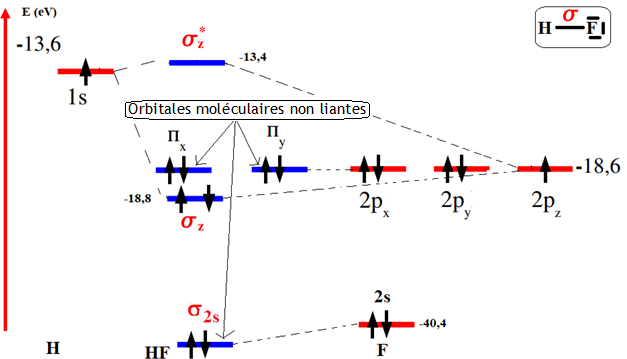
Figure 19. Correlation diagram of HF atomic and molecular energy levels

The electronic configuration of the HF molecule is (σ_1s)² (σ_2s)² (σ_z)² (π_x, π_y)⁴

The H-F molecule has no single electrons, is diamagnetic and has a carbon bond index of 1 (the number of non-bonding electrons is six, bonding electrons and non-bonding electrons is two).^(14,15,41)

The systematic method for constructing Lewis representations⁽³⁶⁾ reveals a single H-F bond and three free pairs on the fluorine atom. We can conclude that the classical model of the systematic method for the construction of Lewis representations confirms and affirms the results we found by the quantum model of molecular orbital theory.⁽⁴²⁾

Case of the H₂O molecule

The H₂O molecule is made up of oxygen as the central atom, whose valence orbitals are s and p, and 2 hydrogen atoms. The oxygen atom is located on all the symmetry elements of the H₂O molecule. The orbital space is based on the four OA of O and the 2 OA 1s of the hydrogens. We will construct the orbital diagram of the H₂O molecule as the result of the interaction of two fragments: O and H₂. The case of the coded H₂O molecule represented in the Oxyz reference frame (figure 20):

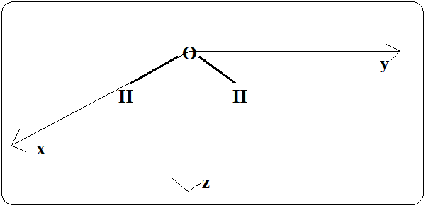
Figure 20. Coordinate system used to define H2O atomic orbitals

We'll consider this planar molecule in the coordinate system shown in figure 20, where all the nuclei lie in the yz plane, and the system's axis of symmetry coincides with the z axis. The minimal basis of the atomic orbitals consists of: the OA 1s(H₁), 1s(H₂) of the two hydrogens, and OA 1s(O), 2s(O), 2p(O) for oxygen.^(43,44,45) The OA 2s of oxygen has an energy of -32,3 eV, while that of the hydrogen atom is -13,6 eV. Given this large energy gap, these two OA do not combine. This AO remains unchanged and simply becomes a non-bonding orbital of the molecule. As oxygen's 2p_x(O) atomic orbital does not overlap with H2's fragment OA (1s(H1) and 1s(H2)), it too becomes a non-bonding orbital. Only the two OAs 2p_z (O) and 2p_y (O) can combine with the two fragment OAs of H₂ to give two bonding molecular orbitals σ_1s-2p_z , σ_1s-2p_y and two other antibonding ones σ_1s-2p_z*, σ_1s-2p_y*.

The symmetry of the system means that these two hydrogen orbitals must be replaced by linear combinations adapted to the symmetry of the H₂O molecule. Note that the electron density is no longer symmetrical between the two atoms. The coefficient of each atom on the OM depends on the energy difference with the OA: the σ_1s-2p_z or σ_1s-2p_y orbital is closer in energy to the 2p(O) orbitals than to the 1s(H) orbital, which is why the coefficient on oxygen is greater than on hydrogen.^(46,47) The oxygen atom therefore has a partial negative charge and the hydrogen a partial positive charge, hence the dipole moment of the H-O bond is 1,5 D ((R_e (H-O)= 0,97Å; E_diss (HO) = 464 Kj/mol; % ionic (HO)= 42,16 %).

Figure 21 shows the orbital energy levels of H₂O, along with their pattern of occupation by the molecule's valence electrons.

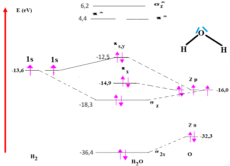
Figure 21. H₂O orbital energy levels and their occupancy pattern by the molecule's valence electrons

The calculated orbitals, in the form of isovalues, are shown in figure 21, highlighting the electronegativity effect. Bonding orbitals are mainly located on the most electronegative atom (O), while antibonding orbitals are located on the least electronegative atoms (H). The eight valence electrons are located in the four lowest-energy OMs in the ground state. There are therefore four bonding electrons corresponding to the two O-H bonds, and four non-bonding electrons corresponding to the two "free pairs" of the classical model representation.⁽³⁶⁾

The electronic configuration of the H₂O molecule is (σ_1s)² (σ_2s)² (σ_1s-2_pz)² (π_x)² (σ_1s-2_py)².^(48,49)

The H₂O molecule has no single electrons, it is diamagnetic, the bonding index of H₂O is 1 (The number of non-bonding electrons is six, bonding electrons or anti-bonding electrons is four).^{(14,15,50,51)}

The systematic method for constructing Lewis representations⁽³⁶⁾ shows a single H-O bond and two free pairs on the oxygen atom. We can conclude that the classical model of the systematic method for the construction of Lewis representations confirms and affirms the results we found by the quantum model of molecular orbital theory.

CONCLUSIONS

LCAO theory is used to calculate molecular orbitals and energies for homonuclear and heteronuclear diatomic molecules. This model can be extended to larger molecules, such as conjugated molecules. This will be dealt with in Huckel's method. In terms of computation time, strong-bond approaches are halfway between ab initio methods such as Density Functional Theory (DFT) or wave functions and force fields. These approaches have been developed in parallel by chemists under the name of Hückel methods or extended Hückel and by physicists under the terminology of strong bonds. (TB for tight binding). Despite the heavy assumptions (no overlap with the neighboring atom) made when applying these methods, satisfactory results can be obtained concerning the characteristics of molecules and their reactivity.

Potential applications of our results, in particular their implications for computer simulations in the following cases: (1) Molecular orbital representations, (2) Schematic molecular orbitals, (3) Density and transparent potential contours, (4) Coordination geometries and polyhedra (5) Coordination polyhedra of molecular complexes, (6) Inorganic structures and crystal stacks, (7) Colored molecular surfaces, (8) Transparent molecular surfaces, (9) Molecular surfaces with color-coded properties (different color scales), and (10) Cut-out molecular surfaces with mapped properties.

The quantum model (molecular orbital theory and hybridization theory) is a fundamental tool for determining the structure and stability of molecules. This model provides a more accurate explanation than the other classical model (Lewis theory and Gillespie theory), especially in complex cases where bonds and interactions have to be evaluated taking electron delocalization into account. This quantum model also helps in various practical applications, such as drug design, where understanding molecular interactions is essential. The classical model of the systematic method for constructing Lewis representations confirms and affirms the results we found by the quantum model of molecular orbital theory of certain molecules namely: O₂, N₂, CO, HF and H₂O.

BIBLIOGRAPHIC REFERENCES

1.  Peter Atkins, Julio de Paula, James Keeler, Atkins' Physical Chemistry, 11th Edition, Oxford University Press; 2002.

2.  P. Chaquin et F. Fuster, OrbiMol, Sorbonne Université, CNRS, Laboratoire de Chimie Théorique (LCT), 75005 Paris (France) ; 2012.

3.  Pierre Grécias, Jean-Pierre Migeon, Chimie Tome 1, Cours Et Tests D'Application, 4éme Edition Broché, Paris, France ; 1995.

4.  Smail Meziane, Chimie générale structure de la matière, 4éme Editions BERTI, Algérie ; 2015.

5.  Yves Jean, Les orbitales moléculaires dans les complexes: cours et exercices corrigés, Editions Ecole Polytechnique, France ; 2003.

6.  P. Chaquin, Y. Canac, C. Lepetit, D Zargarian, R. Chauvin. Estimating local bonding/antibonding character of canonical molecular orbitals from their energy derivatives. The case of coordinating lone pair orbitals. International Journal of Quantum Chemistry, 2016, 116, pp.1285 - 1295.

7.  lattes, G. Montel, introduction à la chimie structurale, Edition Dunod, Paris France ; 1969.

8.  Comninellis, C. K. W. Friedli, A. Sahil-Migirdicyan, Exercices de chimie générale, Collection :Chimie, Laussane, Suisse ; 2018.

9.  Elisabeth Le Masne de Chermont, Arnaud Le Masne de Chermont, Cours de chimie, Éditeur : Heures de France, 2éme édition, France ; 1998.

10.  Maurice Griffé, Chimie, Presses Universitaires De NAMUR, 2éme édition, Belgique ; 2002.

11.  R. Ouahes, B. Devallez, Chimie générale, Edition PUPLISUD, Paris, France ; 1988.

12.  Moszkowicz Pierre, l’atome et la molécule, Alger O. P. U ; 1990.

13.  Le Coarer Jacques, Chimie le minimum à savoir, EDP Sciences, Collection : Grenoble Sciences, France ; 2003.

14.  Alain Sevin, Christine Dézarnaud-Dandine, liaisons chimiques, structure et réactivité, cours et exercices corrigés, Sciences Sup, Dunod, Paris ; 2006.

15.  Yves Jean, Les orbitales moléculaires dans les complexes: cours et exercices corrigés, Editions Ecole Polytechnique, France ; 2003.

16.  Philippe Hiberty et Nguyên Trong Anh, Introduction à la chimie quantique, Éditions École Polytechnique, Paris, France ; 2008.

17.  P. Chaquin et F. Volatron, Chimie Organique. Une approche orbitalaire, DeBoeck; 2015.

18.  Anh N.T., Orbitales frontières, InterEditions-CNRS Editions, Paris ; 1995.

19.  Jean Y., Volatron F., Structure électronique des molécules, Dunod, Paris ; 2003.

20.  Chaquin P., Manuel de Chimie théorique, Ellipses, Paris ; 2000.

21.  Rauk, A., Orbital Interaction Theory of Organic Chemistry, Jonh Wiley & Sons, New- York; 2001.

22.  Fleming, I., Frontier Orbitals and Organic Chemical Reactions, Jonh Wiley & Sons, NewYork; 1970.

23.  Fleming, I., Molecular Orbitals and Organic Chemical Reactions, Jonh Wiley & Sons, NewYork; 2009.

24.  Albright T.A., Burdett J. K., Whangbo M.-H., Orbital Interactions in Chemistry, Jonh Wiley & Sons, New- York; 1985.

25.  D. B. Lawson et J. F. Harrison, « Some Observations on Molecular Orbital Theory », Journal of Chemical Education, vol. 82, no 8, 2005, p. 1205 (DOI 10.1021/ed082p1205).

26.  Catherine E Housecroft, Alan G Sharpe, Chimie inorganique, De Boeck Superieur; 2010.

27.  Bickelhaupt F.M., Nagle J.K., Klemm W.L., Role of s-p orbital mixing in the bonding and properties of the second-period diatomic molecules, J. Phys. Chem. A, 2008, 112, p. 2437.

28.  Robinson P.J., Alexandrova A.N., Assessing the bonding properties of individual molecular orbitals, J. Phys. Chem. A, 2015, 119, p. 12862.

29.  Chaquin P., Canac Y., Lepetit C., Zargarian D., Chauvin R., Estimating local bonding/antibonding character of canonical molecular orbitals from their energy derivatives: the case of coordinating lone pair orbitals, Int. J. Quant. Chem., 2016, 116, p. 1285.

30.  Chaquin P., Fuster F., Bonding/antibonding character of “lone pair” molecular orbitals in small molecules (AH, AH2, AH3, AF3 and H2CO) from their energy derivatives; consequences for experimental data, ChemPhysChem, 2017, 18, p. 2873.

31.  Fuster F, Chaquin P., Analysis of carbon-carbon bonding in small hydrocarbons and dicarbon using dynamic orbital forces: bond energies and sigma/pi partition. Comparison with sila compounds, Int. J. Quantum Chem., 2019, 119, e25996.

32.  Chaquin P., Gutlé C., Reinhardt P., (2014) Liaison(s) chimique(s) : forces ou énergie ? En tout cas, électrostatique, L’Act. Chim., 384, p. 29.

33.  Berlin T.J., (1951) Binding regions in diatomic molecules, Chem. Phys., 19, p. 208.

34.  Averill F.W., Painter G.S., (1986) Orbital forces and chemical bonding in density-functional theory: application to first-row dimers, Phys. Rev. B, 34, p. 2088.

35.  Tal T., Katriel J., (1977) Bonding criteria for diatomic molecular orbitals and relations among them, Theoret. Chim. Acta, 46, p. 173.

36.  Lahbib Abbas, Lahcen Bih, Khalid Yamni, Abderrahim Elyahyaouy, Abdelmalik El Attaoui, Zahra Ramzi, Systematic Method for Constructing Lewis Representations, , Open Journal of Inorganic Chemistry Vol.14 No.1, January 31, 2024, DOI: 10.4236/ojic.2024.141001.

37.  Pauling L., The Nature of the Chemical Bond and the Structure of Molecules and Crystals: an Introduction to Modern Structural Chemistry, 3e ed., Cornell University Press; 1960.

38.  Frey, Paul Reheard, College chemistry [archive], 3e éd., Prentice-Hall, Université de Californie; 1965.

39.  Alcock, N.W., Bonding and Structure: structural principles in inorganic and organic chemistry, Ellis Horwood Ltd; 1ère edition, New York; 1990.

40.  Werner Kutzelnigg, Einführung in die Theoretische Chemie, Weinheim, Wiley-VCH, décembre 2001, 896 p. (ISBN 3527306099).

41.  J.S. Baskin and A.H. Zewail. Freezing atoms in motion: Principles of femtochemistry and demonstration by laser spectroscopy, Journal of Chemical Education, 78:737, 2001.

42.  A.D. Bandrauk and H. Shen. Exponential split operator methods for solving coupled time dependent Schroedinger equations, Journal of Chemical Physics, 99:1185, 1993.

43.  H.-Z. Lu and A.D. Bandrauk. Moving adaptive grid methods for numerical solution of the time dependent molecular Schroedinger equation in laser fields, Journal of Chemical Physics, 115:1670, 2001.

44.  E. H. Hückel. Z. Phys., 70 :204–86, 1931.

45.  Max Wolfsberg and Lindsay Helmholz. The spectra and electronic structure of the tetrahedral ions MnO4, Cro4, and ClO4. J. Chem. Phys., 20 :837–843, 1952.

46.  R. Hoffmann. An extended hückel theory. i. hydrocarbons. J. Chem. Phys., 39 :1397–16, 1963.

47.  R. Hoffmann. Extended hückel theory. iii. compounds of boron and nitrogen. J. Chem. Phys., 40 :2474–7, 1964.

48.  R. Hoffmann. Extended hückel theory—v : Cumulenes, polyenes, polyacetylenes and Cn. Tetrahedron, 22 :521–538, 1966.

49.  D. J. Chadi. (110) surface atomic structures of covalent and ionic semiconductors. Phys. Rev.B, 19 :2074—2082, 1979.

50.  W. A. Harrison. Electronic structure and the properties of solids, W. H. Freeman ed., San Francisco; 1980.

51.  J. Friedel. The physics of metals, J. M. Ziman, Cambridge University Press, Cambridge; 1969.

FINANCING

The authors declare that they have no known competing financial interests or personal relationships that could have appeared to influence the work reported in this paper.

CONFLICT OF INTEREST

The authors declare that there is no conflict of interest.

AUTHORSHIP CONTRIBUTION

Conceptualization: Abdessamad MEZDAR, Khalid SELLAM, Ilyas. JALAFI, Zahra RAMZI.

Data curation: Lahbib ABBAS, Lahcen BIH.

Formal analysis: Khalid SELLAM, Ilyas. JALAFI, Zahra RAMZI.

Research: Abdessamad MEZDAR, Ilyas. JALAFI, Zahra RAMZI.

Methodology: Lahbib ABBAS, Lahcen BIH.

Project management: Zahra RAMZI.

Resources: Lahbib ABBAS.

Software: Lahbib ABBAS, Lahcen BIH.

Supervision: Lahbib ABBAS, Lahcen BIH.

Validation: Lahbib ABBAS, Lahcen BIH.

Display: Lahbib ABBAS, Lahcen BIH.

Drafting - original draft: Abdessamad MEZDAR, Khalid SELLAM, Ilyas. JALAFI, Zahra RAMZI.